Section 4.3 The Chromatic Polynomial
Subsection 4.3.1 History
During the period that the Four-Color Theorem was unsolved, which spanned more than a century, mathematicians from around the globe introduced numerous approaches with the hope to find a solution. One approach noted that the number of ways a map can be colored using \(\lambda\) colors has a polynomial dependence on \(\lambda\text{.}\)
By viewing maps as loop-less planar graphs, in 1912, George David Birkhoff defined a function \(P(M,\lambda)\) that produces the number of proper \(\lambda\)-colorings of a map \(M\) for a positive integer \(\lambda\) and called it the chromatic polynomial of \(M\text{.}\) Consequently, if he could verify that \(P(M, 4) \gt 0\) for every loop-less planer map \(M\text{,}\) then he would prove the Four-Color Theorem.
Although he was unsuccessful in this attempt, chromatic polynomials became an important mathematical tool in algebraic graph theory and continues to be a subject of great interest. Birkhoff’s definition is limited in that it only defines chromatic polynomials for loop-less planar graphs. The concept of chromatic polynomials was extended in by Hassler Whiteney in 1932 to graphs which cannot be embedded into the plane.
Subsection 4.3.2 Introduction
Definition 4.3.1.
For a graph \(G\) and a positive integer \(\lambda\) the number of different proper \(\lambda\)-colorings of \(G\) is denoted by \(P(G, \lambda)\) and is called the Chromatic Polynomial of \(G\text{.}\)
A Simple Graph is an undirected graph containing no edges connecting a vertex to itself and contains at most one edge between any two adjacent vertices.
We can see that if \(\lambda \lt \chi (G)\text{,}\) since there are no possible \(\lambda\)-colorings of the graph, \(P(G,\lambda)=0\text{.}\)
Theorem 4.3.2.
The chromatic function of a simple graph is a polynomial
Proof.
Construct proper colorings of \(G\) by partitioning \(V(G)\) into disjoint sets and assigning a unique color to each disjoint set. A disjoint set is a set of vertices in which no two vertices in the same set are adjacent. Given \(\lambda\) colors, there will be \(\lambda\) ways to choose the color for the first set, \((\lambda - 1)\) ways to choose the color for the second set, \((\lambda - 2)\) ways to choose the color for the third set, and so on. There are then \(\lambda(\lambda -1)(\lambda -2)...\) possible ways to color the vertices of graph \(G\) such that they result in a proper coloring, and it is clear that this is some polynomial.
Subsection 4.3.3 Types of GraphsThe Chromatic Polynomial of More Complicated Graphs
Proposition 4.3.3.
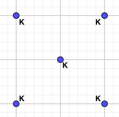
The chromatic polynomial of a Collection of Vertices on \(n\) vertices is \(P(G,\lambda)=\lambda^n\)
Proof.
Let G be a Collection of Vertices (i.e. \(n\) vertices and no edges). Since no vertex is adjacent to any other vertex in the graph, there are \(\lambda\) ways to color each vertex, so \(P(G,\lambda)=\lambda^n\text{.}\)
Proposition 4.3.4.
The chromatic polynomial of a Path on \(n\) vertices is \(P(G,\lambda)=\lambda(\lambda-1)^{n-1}\)
Proof.
Let G be a path on \(n\) vertices (\(V=\{x-1, x_2,..., x_n\}, E=\{x_ix_{i+1}\}\)) and begin by coloring \(x_1\text{.}\) There are \(\lambda\) choices of color for \(x_1\text{,}\) and \((\lambda-1)\) choices of color for the \(x_2\) because it is adjacent to the \(x_1\text{.}\) For \(x_3\text{,}\) we also have \((\lambda-1)\) choices of color because it is only adjacent to \(x_2\text{.}\) Similarly, we will have \((\lambda-1)\) choices of color for all of the remaining vertices, meaning \(P(G,\lambda)=\lambda(\lambda-1)^{n-1}\text{.}\)
Example 4.3.5.
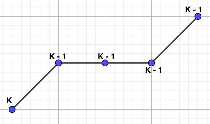
To color the following graph with \(k\) colors notice that the color of the first vertex does not matter, we can choose any of the \(k\) colors. Then for the next vertex in the line we need to ensure that we do not pick the same color as the first vertex. Leaving us with \(k-1\) choices for the color of the second vertex. For the third vertex we only need to worry about not coloring it with the color of the second vertex. So on and so forth until we have that the chromatic
Proposition 4.3.6.
The chromatic polynomial of a Tree on \(n\) vertices is \(P(G,\lambda)=\lambda(\lambda-1)^{n-1}\)
Proof.
Consider a proof by induction;
Base Case: Let \(n = 1\text{.}\) The claim clearly holds as we have \(\lambda\) choices of color for the one vertex.
Inductive Step: Assume that the claim holds for a graph on \(n\) vertices. Select any leaf and prune it from the tree. The chromatic polynomial for the resulting tree will be \(\lambda(\lambda-1)^{n-2}\) by assumption. Now, replace the pruned leaf. We can assign any color to this vertex except for that of its neighbour, and thus have \((\lambda-1)\) choices of color. Therefore the chromatic polynomial of Tree is \(P(G,\lambda)=\lambda(\lambda-1)^{n-1}\text{.}\)
Example 4.3.7.
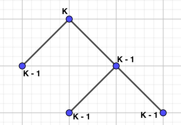
Suppose we want to color this tree with \(k\) colors. Starting with the root of the tree, we can color this vertex with \(k\) colors. Then for each adjacent vertex we must make sure we do not color those vertices with the same color as the root of the tree. So, each of these vertices can be colored with \(k-1\) colors. Moving down the tree, to the last remaining not colored vertices, we notice that the only vertex that we need to be a different color is their shared adjacent vertex. Hence, each of these last two vertices can be colored with \(k-1\) colors. The chromatic polynomial then becomes \(k(k-1)(k-1)(k-1)(k-1)=k(k-1)^4\text{.}\)
Proposition 4.3.8.
The chromatic polynomial of a Complete Graph on \(n\) vertices is \(P(G,\lambda)=\lambda(\lambda-1)(\lambda-2)...(\lambda-n+1)=\frac{\lambda!}{(\lambda-n)!}\)
Proof.
Let G be a Complete Graph on \(n\) vertices. We can choose any of the \(\lambda\) colors for the first vertex we color. For the second vertex we color, we have \((\lambda-1)\) choices since it is adjacent to first vertex. Now since each vertex is adjacent to the rest, we have \((\lambda-2)\) choices of color for the third vertex we color, and so on. This yields a polynomial \(\lambda(\lambda-1)(\lambda-2)\text{...,}\) but terminates later when we reach the \(n^{th}\) vertex. If we follow our process for choosing colors, the number of colors we will have available for the last vertex will be \((\lambda-n+1)\text{,}\) because we started at \(\lambda\) and we counted down \((n-1)\) terms. Therefore \(P(G,\lambda)=\lambda(\lambda-1)(\lambda-2)...(\lambda-n+1)=\frac{\lambda!}{(\lambda-n)!}\text{.}\)
Example 4.3.9.
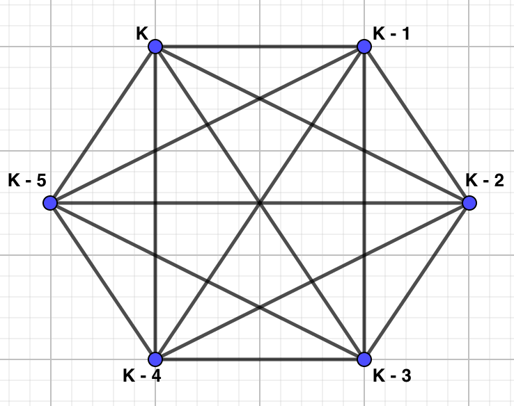
For this example, let us color a complete graph with 5 vertices with \(k\) colors. Pick any vertex to start with, we have \(k\) colors to choose from. Then move onto the adjacent vertex clockwise in the graph. This vertex cannot be colored the same color as the first vertex, so we have \(k-1\) colors to choose from. Again moving to the next adjacent vertex clockwise around the graph, we see that we cannot color this vertex with the first or second color because this third vertex is adjacent to both the first and second vertices, hence, this third vertex can be colored with only \(k-2\) colors. Continuing this process our chromatic polynomial becomes \(k(k-1)(k-2)(k-3)(k-4)\text{.}\)
Calculating the chromatic polynomial of a graph is not always as straightforward as with the families of graphs shown above. The choice of how to color a graph while minimizing the number of colors used can actually be very complex. Therefore, we need a method where we can consistently obtain the chromatic polynomial of any graph. And so, in 1977 Paul Erdos and Robin J. Wilson made note of what we now refer to as the Deletion-Contraction property. The Deletion-Contraction property can be very useful in breaking down the problem into parts which are much easier to solve.
Definition 4.3.10.
Consider a graph \(G\) with an edge \(e\) and its associated vertices \(u\) and \(v\text{.}\) Let \(G-e\) be the graph without \(e\) and let \(G/e\) be the graph \(G\) where \(e\) is removed, and \(u\) and \(v\) are combined into a single vertex. We call \(G-e\) the deletion of \(e\) and \(G/e\) the contraction of \(e\text{.}\)
Theorem 4.3.11.
Deletion-Contraction Property: For a graph \(G\text{,}\) one of its edges \(e\text{,}\) and \(\lambda\) colors,the chromatic polynomial of \(G\) is \(P(G, \lambda)=P(G-e, \lambda)-P(G/e, \lambda)\)
Proof.
Consider a graph \(G\) and one of its edges \(e\text{.}\) Let \(u\) and \(v\) be the two vertices connected to \(e\text{.}\) To be a proper coloring, \(u\) and \(v\) must be colored different colors. In the graph \(G/e\text{,}\) \(u\) and \(v\) are represented by a single vertex, and so, they have the same color. In the graph \(G-e\text{,}\) \(u\) and \(v\) are no longer adjacent, and so they could be colored with the same color or different colors, they are no longer related. This means the number of colorings of \(G-e\) is the same as the total number of colorings of \(G\) and \(G/e\text{.}\) Therefore, \(P(G-e, \lambda)=P(G, \lambda)+P(G/e, \lambda)\) or with some rearranging, \(P(G, \lambda)=P(G-e, \lambda)-P(G/e, \lambda)\text{.}\)
Theorem 4.3.12.
Any graph with clique size \(k\) requires at least \(k\) colors for a proper coloring.
Proof.
A clique is defined as a subset of vertices such that every pair of vertices in the subset is adjacent. Another way to think of this is that the induced subgraph is complete. Each vertex within the clique is adjacent to \(k-1\) other vertices which are all in turn adjacent to other \(k-1\) vertices in the clique. By the definition of a proper coloring, the colors assigned to each of the vertices in such a clique, including the original vertex must be all distinct. Hence if we have a click of size \(k\text{,}\) there must be \(k\) colors in the proper coloring.
Subsection 4.3.4 Examples
Example 4.3.13.
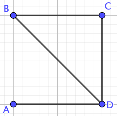
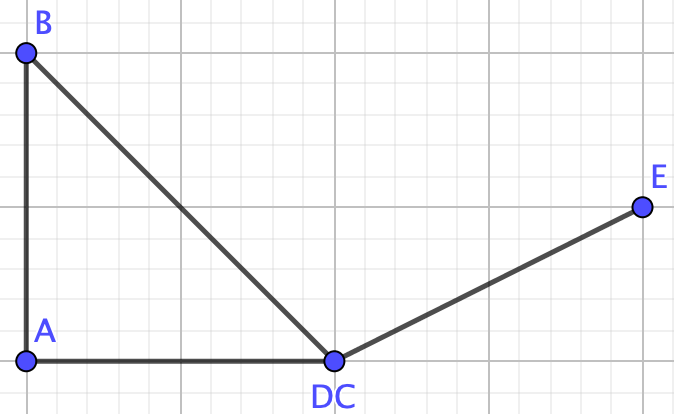
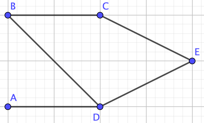
Find the chromatic polynomial of the following graph with \(\lambda\) colors.
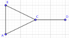
First, notice that this graph is not a collection of nodes, a path, a tree, or a complete graph therefore we cannot use any of the formulas we proved above. We need the deletion-contraction property! We can choose any edge that we want, there is some strategy to picking which edge to remove so you have less steps, but any edge will so. So, remove edge \(BC\) leaving us with the graph \(G-e\)
Example 4.3.14.
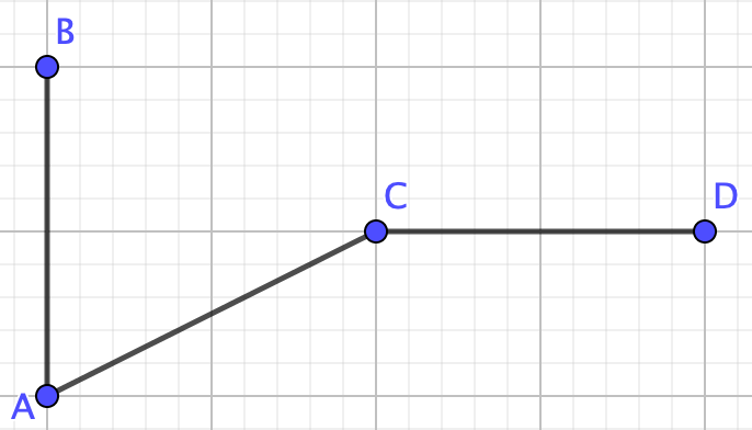
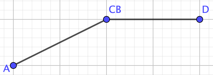
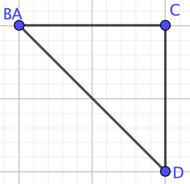
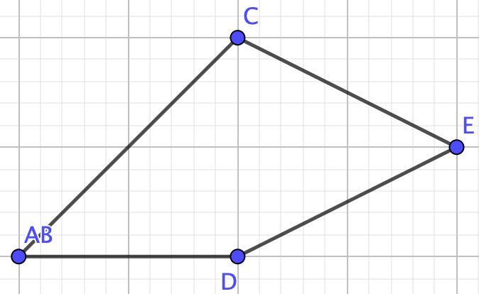
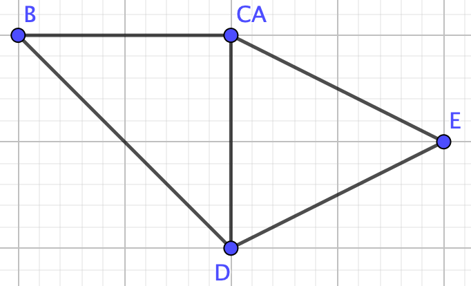
Find the chromatic polynomial of the following graph with \(\lambda\) colors.
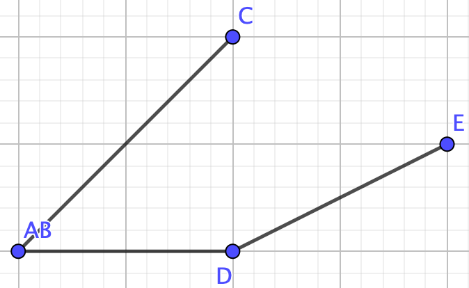
Again, notice that this graph is not a collection of nodes, a path, a tree, or a complete graph therefore we cannot use any of the formulas we proved above. We need the deletion-contraction property. So, let us remove edge \(AB\) leaving us with graph \(G-e\text{.}\)
Example 4.3.15.
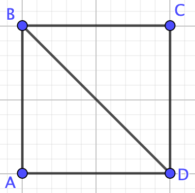
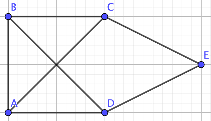
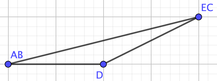
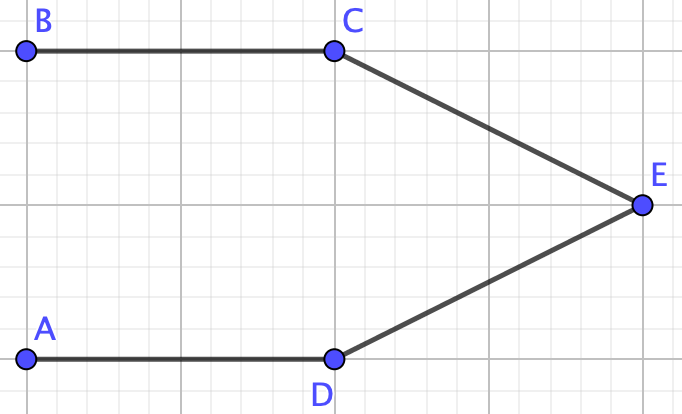
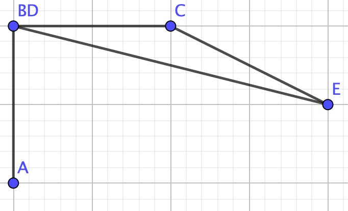
Find the chromatic polynomial of the following graph with \(\lambda\) colors.
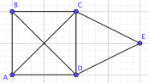
Graph \(G\) is not a collection of nodes, a path, a tree, or a complete graph therefore we cannot use any of the formulas we proved above. We need the deletion-contraction property!So, remove edge \(CD\) to make graph \(G_1-e\)

\(P(G_5-e,\lambda)-P(G_5/e,\lambda)=P(G_4-e,\lambda)\) \(\lambda^5-4\lambda^4+6\lambda^3-4\lambda^2+\lambda-[\lambda^4-4\lambda^3+5\lambda^2-2\lambda]=\lambda^5-5\lambda^4+10\lambda^3-9\lambda^2+3\lambda\) \(P(G_4-e,\lambda)-P(G_4/e,\lambda)=P(G_2-e,\lambda)\) \(\lambda^5-5\lambda^4+10\lambda^3-9\lambda^2+3\lambda-[\lambda^4-5\lambda^3+8\lambda^2-4\lambda]=\lambda^5-6\lambda^4+15\lambda^3-17\lambda^2+7\lambda\) \(P(G_3-e,\lambda)-P(G_3/e,\lambda)=P(G_2/e,\lambda)\) \(\lambda^4-3\lambda^3+3\lambda^2-\lambda-[\lambda^3-3\lambda^2+2\lambda]=\lambda^4-4\lambda^3+6\lambda^2-3\lambda\) \(P(G_2-e,\lambda)-P(G_2/e,\lambda)=P(G_1-e,\lambda)\) \(\lambda^5-6\lambda^4+15\lambda^3-17\lambda^2+7\lambda-[\lambda^4-4\lambda^3+6\lambda^2-3\lambda]=\lambda^5-7\lambda^4+19\lambda^3-23\lambda^2+10\lambda\) \(P(G_1-e,\lambda)-P(G_1/e,\lambda)=P(G,\lambda)\) \(\lambda^5-7\lambda^4+19\lambda^3-23\lambda^2+10\lambda-[\lambda^4-4\lambda^3+5\lambda^2-2\lambda]=\lambda^5-8\lambda^4+23\lambda^3-28\lambda^2+12\lambda\)
Subsection 4.3.5 Which Polynomials Are Chromatic
In this section we will prove various properties surrounding chromatic polynomials, in particular their coefficients and their roots.
Theorem 4.3.16.
The lead coefficient of \(P(G,\lambda)\) must always be one.
Proof.
Suppose that \(G\) has \(n\) vertices. We will proceed by induction on the number of edges.
Base case: Let \(G\) have only one edge. Then the \(n-2\) vertices with no edges can be colored with any of our \(\lambda\) colors, and the two vertices on the edge can be colored in \(\lambda(\lambda-1)\) ways, so, \(P(G,\lambda)=\lambda^{n}-\lambda^{n-1}\text{.}\) So, the leading coefficient of \(P(G,\lambda)\) is one.
Inductive Step: We will proceed with strong induction. Assume that the statement is true for all graphs with fewer than \(k\) edges. Assume that \(G\) has \(k\) edges and let \(\beta \in E(G)\) be one of them. By the deletion-contraction property, \(P(G,\lambda)=P(G-\beta, \lambda)-P(G/\beta, \lambda)\text{.}\) Now, since \(G-\beta\) has fewer than \(k\) edges, by the induction hypothesis, \(P(G-\beta, \lambda)\) has a lead coefficent of one and degree \(n\text{.}\) Since \(G/\beta\) has fewer than \(k\) edges and only \(n-1\) vertices, \(P(G/\beta, \lambda)\) also has a lead coefficent of one, but degree \(n-1\text{.}\) Upon subtraction of these polynomials, we see that the lead term is the same lead term as that in \(P(G-\beta), \lambda)\text{,}\) so the lead coeffienct of \(P(G,\lambda\) is one. Therefore, by induction, the statement is true for all graphs with \(n\) vertices and any number of edges.
Theorem 4.3.17.
The coefficient of the second term of \(P(G,\lambda)\) is \(|E(G)|\text{.}\)
Proof.
Again, we will proceed by induction on the number of edges of \(G\text{.}\)
Base Case: As in the proofs of the above theorems, let \(G\) have only one edge. Then the \(n-2\) vertices with no edges can be colored with any of our \(\lambda\) colors, and the two vertices on the edge can be colored in \(\lambda(\lambda-1)\) ways, so, \(P(G,\lambda)=\lambda^{n}-\lambda^{n-1}\text{.}\) So, the coefficient of the second term of \(P(G,\lambda)\) is one, so our statement is true for our base case.
Inductive Step: Again, we will proceed using strong induction. Assume the statement is true for all graphs on \(n\) vertices with fewer than \(k\) edges. Let \(G\) be a graph with \(k\) edges and consider the deletion-contraction property. Since \(G-\beta\) and \(G/\beta\) both have fewer than \(k\) edges, we can apply our induction hypothesis and assume that their chromatic polynomials have the following form: \(P(G-\beta, \lambda)=\lambda^n-a_{n-1}\lambda^{n-1}+a_{n-2}\lambda^{n-2}-...\text{,}\) and \(P(G/\beta, \lambda)=\lambda^{n-1}-b_{n-2}\lambda^{n-2}+b_{n-3}\lambda^{n-3}-...\text{,}\) where \(a_{n-1}\) is the number of edges in \(G-\beta\) and \(b_{n-2}\) is the number of edges in \(G/\beta\text{.}\) Now since \(P(G,\lambda)=P(G-\beta, \lambda)-P(G/\beta, \lambda)\text{,}\) by the deletion contraction property;
\(P(G,\lambda)=(\lambda^n-a_{n-1}\lambda^{n-1}+a_{n-2}\lambda^{n-2}-...)-(\lambda^{n-1}-b_{n-2}\lambda^{n-2}+b_{n-3}\lambda^{n-3}-...)\)
\(P(G,\lambda)=\lambda^n-(a_{n-1}+1)\lambda^{n-1}+(a_{n-2}+b_{n-2})\lambda^{n-2}-...\)
Now since \(G-\beta\) is obtained from \(G\) by the removal of one edge, \(a_{n-1} = (k - 1)\text{,}\) so \(a_{n-1}+1 = k\text{,}\) and the statement is true. Therefore by induction, the statement is true for all graphs with \(n\) vertices and any number of edges.
Theorem 4.3.18.
The constant term, i.e. the coefficient of 1 in \(P(G,\lambda)\) is always zero
Proof.
We know that \(P(G,0)\) is the number of ways to color the graph \(G\) with no colors. But a graph cannot be colored with no colors, so \(a_0=0\text{.}\)
Theorem 4.3.19.
The coefficients of the chromatic polynomial alternate in sign.
Proof.
(By Strong Induction) We want to show that the statement is true for all graphs, so we will use induction on the number of edges in the graph to do so.
Base Case: If our graph has a single edge, then the chromatic polynomial of the graph with \(n\) and one edge is \(x^n-x^{n-1}\text{.}\) This has alternating signs, so our base case holds.
Now suppose this statement holds for all graphs with fewer than \(k\) edges. Now we want to show that the statement holds true for a graph with \(k\) edges.
We know from the deletion-contraction theorem that \(P(G_k,\lambda)=P(G_k-e,\lambda)-P(G_k/e,\lambda)\text{.}\) Now since both \(P(G_k-e,\lambda)\) and \(P(G_k/e,\lambda)\) both have \(k-1\) edges, our induction hypothesis holds for both of these graphs, so they take the form
\(P(G_k-e,\lambda)=\lambda^n-a_{n-1}\lambda^{n-1}+a_{n-2}\lambda^{n-2}-\cdots\)
\(P(G_k/e,\lambda)=\lambda^{n-1}-b_{n-2}\lambda^{n-2}+b_{n-3}\lambda^{n-3}-\cdots\)
So by our deletion contraction theorem we have that
\(P(G_k,\lambda)=(\lambda^n-a_{n-1}\lambda^{n-1}+a_{n-2}\lambda^{n-2}-\cdots)-(\lambda^{n-1}-b_{n-2}\lambda^{n-2}+b_{n-3}\lambda^{n-3}-\cdots)\)
\(\lambda^n-(a_{n-1}+1)\lambda^{n-1}+(a_{n-2}+b_{n-2})\lambda^{n-2}-\cdots\)
Thus, the signs alternate for a graph with \(k\) edges, so our statement is true for all graphs.
Theorem 4.3.20.
For a connected graph, the coeffecients satisfy \(1=|a_n|\lt |a_{n-1}|\lt \cdots \lt \left|a_{\left[\frac{n}{2}\right]+1}\right|\)
Proof.
We want to show that \(|a_{m+1}|\lt |a_m|\) for all \(m\gt \frac{n}{2}\)
Case 1: Let \(G\) be a tree \(T_n\) From previous proofs we know that for a graph of a tree \(P(T_n,\lambda)=\lambda(\lambda-1)^{n-1}\) so we have that \(a_{m}=(-1)^{n-m}\binom{n-1}{m-1}\) and thus we need to show that \(\binom{n-1}{m}\lt \binom{n-1}{m-1}\)
So we need to show that \(\frac{(n-1)!}{m!(n-m-1)!}\lt \frac{(n-1)!}{(m-1)!(n-m)!}\) then since by our statements regarding \(n\) and \(m\) we know that \(n-m\lt m\) so we have
\(n-m\lt m\) which tells us that
\(m!(n-m-1)!\gt (m-1)!(n+1)!\) so we have
\(\frac{(n-1)!}{m!(n-m-1)!}\lt \frac{(n-1)!}{(m-1)!(n-m)!}\)
Thus the inequality holds
Case 2: If \(G\) is not a tree, then we can use an iterative application of the deletion-contraction theorem along with the following theorem 4.3.19 to prove the inequality.
If \(G\) is not a tree then remove edge \(e\) where \(e\) is an edge that is part of a cycle. Then by the deletion contraction theorem and theorem 4.3.19 that we subtract the polynomials, and since the signs of the corresponding coefficients alternate we know the corresponding coefficients will add their absolute values. So the contracted graph will have
\(0=|a'_n|\lt 1=|a'_{n-1}|\lt |a'_{n-2}|\lt \cdots \left|a'_{\frac{n-1}{2}+1}\right|\)
So since their absolute values add up, and since \(G-e\) and \(G/e\) both satisfy the inequalities, the inequality also holds for the graph \(G\text{.}\)
Theorem 4.3.21.
A chromatic polynomial has no negative real roots
Proof.
Because we know from theorem 4.3.19 that the coefficients of a chromatic polynomial alternate in sign, we know our chromatic polynomial takes the form
\(P(G,\lambda)=\sum \limits_{m=1}^{n} a_m\lambda^m\)
where \(a_m\ge 0\) if \(n\equiv m \mod 2\) (since the polynomial alternates in sign). Then if we multiply \((-1)^nP(G,\lambda)\text{,}\) this quantity will be greater than or equal to zero if \(\lambda\lt 0\text{.}\) So it remains to show that it cannot be equal to zero. Since we know that \(a_n=1>0\text{,}\) we know that \((-1)^nP(G,\lambda)\gt 0\text{.}\) So this product is strictly greater than zero, Thus, no negative value of \(q\) can be a root of the chromatic polynomial.
There are many similar properties of chromatic polynomials that can be proven surrounding the coefficients and roots of the chromatic polynomials. However there are still properties left to be proven. So far we have proven that the coefficients of a chromatic polynomial are increasing in absolute value up to the \(\frac{n-1}{2}+1\) coefficient. An extension of this is called the Unimodal conjecture which states:
Proposition 4.3.22.
There exists some \(k\) such that
\(0=|a_n|\le|a_{n-1}|\le\cdots\le |a_{k+1}|\le|a_k|\ge|a_{k-1}|\ge\cdots\ge|a_2|\ge|a_1|\)
This claim has been proven for specific types of graphs but has not been proven in the general case. In the following section we will find that there are other aspects of chromatic polynomials that seem like they should be true, but aren't or haven't been proven.
Subsection 4.3.6 Open Questions
When given any polynomial, how can we determine whether or not there exists a graph for which this polynomial is the chromatic polynomial? While we have a necessary set of conditions that we can check a given polynomial against there is still no set of sufficient conditions! For example, consider the following polynomial:
Notice that we can factor this polynomial into \(k^2(k-1)(k-2)\text{.}\) There are two vertices with \(x\) choices of colors because of the \(k^2\text{,}\) so the graph necessarily has two components. From Theorem ADD the absolute value of the coefficients of the \(x^3\)term is 4 so the graph must have 4 edges. Since \(|E|\) is 4 and there must be two components, the most edges we could have in a simple graph would be 3, and that would result in an isolated vertex. The only other option would be two vertices in each component (which would not make sense with this chromatic polynomial) and then the graph would only have two edges. Therefore, it is impossible to have a connected graph on 4 vertices with this chromatic polynomial, and there are too many edges for there to be a disconnected graph with this chromatic polynomial. So, even though this seemingly innocent polynomial meets several of our above Theorems, it is not the chromatic polynomial of a graph.